How To Draw Root Locus
How To Draw Root Locus - Symmetrical about the real axis rule 3: Web this page was developed to help student learn how to sketch the root locus by hand. All the root loci starts from the poles where k = 0 and terminates at the zeros where k tends to infinity. Web in this article, we will walk you through the steps involved in drawing the root locus of a system. Web sketching root locus part 1 brian douglas 282k subscribers subscribe subscribed 10k 760k views 10 years ago classical control theory, section 2: This web page attempts to demystify the process. Root locus sketching rules negative feedback rule 1: Os ≤ 10% (ζ ≥ 0.59), ts ≤. Web the matlab control systems toolbox provides the ‘rlocus’ command to plot the root locus of the loop transfer function. Web rlocus (sys) calculates and plots the root locus of the siso model sys.
That is, number of poles of f(s). There are many systems where relative stability as a function of some parameter other than gain is required. Web rule 1 − locate the open loop poles and zeros in the ‘s’ plane. Web the matlab control systems toolbox provides the ‘rlocus’ command to plot the root locus of the loop transfer function. The following example compares the root locus design of analog and digital controllers in the case of a dc motor model. Web 125 share 5.9k views 1 year ago in this video, i go over a general method for drawing a root locus diagram. The ‘rlocus’ command is invoked after defining a dynamic system object using ‘tf’ or ‘zpk’ command.
Web procedure to plot root locus find out all the roots and poles from the open loop transfer function and then plot them on the complex plane. N(s) has zeros at z. Web rlocus (sys) calculates and plots the root locus of the siso model sys. The ‘rlocus’ command is invoked after defining a dynamic system object using ‘tf’ or ‘zpk’ command. D(s) is n th order:
Examples on Sketching Root Locus YouTube

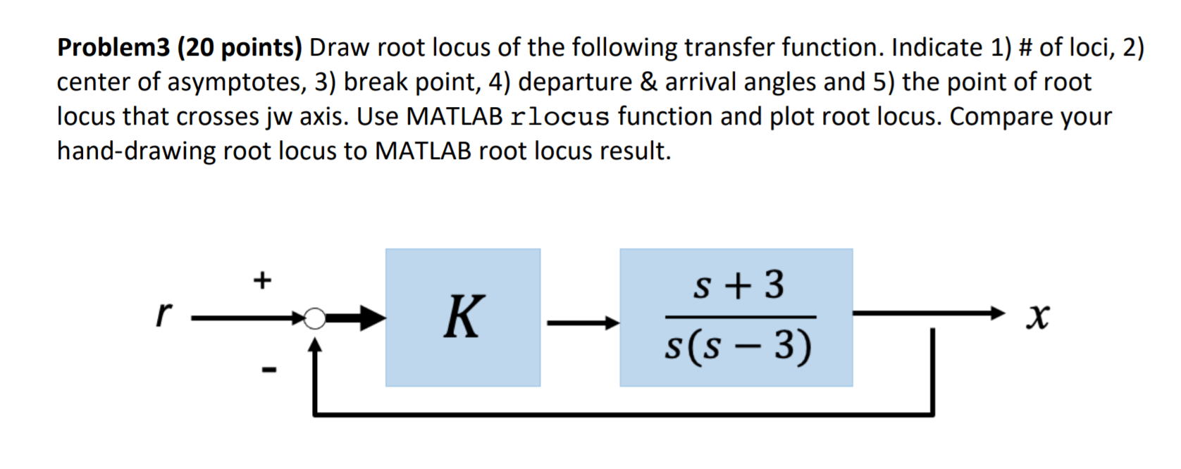
Solved Draw root locus of the following transfer function.
3.3 Root Locus Sketching (Part 1) YouTube

How to Draw Root Locus of a System? ShortsFlood

Solved Draw the root locus of the following systems. G(s) =

How to Draw a Root Locus of a System? DataFlair

Solved 2. (25) Draw the rootlocus diagrams for the

Properties of open loop gain used to draw root locus. Simple integrator has one pole. Symmetrical about the real axis rule 3: Web rule 1 − locate the open loop poles and zeros in the ‘s’ plane. The ‘rlocus’ command is invoked after defining a dynamic system object using ‘tf’ or ‘zpk’ command. Web in this article, we will walk you through the steps involved in drawing the root locus of a system.
The loop gain is kg(s)h(s) which can be rewritten as kn(s)/d(s). Web the matlab control systems toolbox provides the ‘rlocus’ command to plot the root locus of the loop transfer function. Os ≤ 10% (ζ ≥ 0.59), ts ≤. Root locus sketching rules negative feedback rule 1: Web learn the first and the simplest rule for drawing the root locus.
G(s) = 500 s2 + 110s + 1025; Here three examples are considered. Web general steps to draw root locus 1. Web rule 1 − locate the open loop poles and zeros in the ‘s’ plane.
Web Rlocus (Sys) Calculates And Plots The Root Locus Of The Siso Model Sys.
Root locus sketching rules negative feedback rule 1: There are many systems where relative stability as a function of some parameter other than gain is required. K>0, a 0 >0, b 0 >0. N(s), the numerator polynomial, is m th order;
All The Root Loci Starts From The Poles Where K = 0 And Terminates At The Zeros Where K Tends To Infinity.
This web page attempts to demystify the process. That is, number of poles of f(s). Web about press copyright contact us creators advertise developers terms privacy policy & safety how youtube works test new features nfl sunday ticket press copyright. This is not the only way that the diagram can be drawn, but i found that these.
G(S) = 500 S2 + 110S + 1025;
Get the map of control theory:. Simple integrator has one pole. Web the matlab control systems toolbox provides the ‘rlocus’ command to plot the root locus of the loop transfer function. Therefore there are 2 branches to the locus.
Properties Of Open Loop Gain Used To Draw Root Locus.
The ‘rlocus’ command is invoked after defining a dynamic system object using ‘tf’ or ‘zpk’ command. The loop gain is kg(s)h(s) which can be rewritten as kn(s)/d(s). Web procedure to plot root locus find out all the roots and poles from the open loop transfer function and then plot them on the complex plane. We know that the root locus branches start at the open loop poles and end at open loop zeros.